How the Self-Driving Tech Stack Works

How the Self-Driving Tech Stack Works
Most explanations of self-driving cars wave their hands at "AI" and "sensors." This isn't that. This is a walk through the actual software stack—from raw sensor data to wheel actuation—with code from real open source implementations.
We'll examine two primary open source stacks: comma.ai's openpilot (end-to-end neural network approach) and Autoware (modular ROS2-based stack). These represent the two dominant architectural philosophies in autonomous driving.
The Hardware Layer
Sensor Suite
Every autonomous vehicle starts with sensors. The choice of sensors defines the capabilities and constraints of the entire system.
| Sensor | Data Rate | Resolution | Range | Use Case |
|---|---|---|---|---|
| Camera | 20-60 Hz | 1-8 MP | ~200m | Lane detection, sign recognition, object classification |
| LiDAR | 10-20 Hz | 64-128 channels | ~200m | 3D point cloud, precise distance measurement |
| Radar | 10-20 Hz | Low | ~250m | Velocity measurement, all-weather operation |
| IMU | 100-200 Hz | N/A | N/A | Acceleration, rotation rates |
| GNSS/GPS | 1-10 Hz | ~2m accuracy | Global | Absolute positioning |
| Wheel Odometry | 50-100 Hz | N/A | N/A | Velocity, distance traveled |
openpilot's approach is notably camera-only (plus IMU). No LiDAR, no radar dependency. This mirrors Tesla's vision-only philosophy and is enabled by advances in neural network perception.
Autoware is sensor-agnostic but typically deploys with LiDAR + camera fusion, following the traditional robotics approach of redundant sensing modalities.
The comma 3X Hardware
openpilot runs on the comma 3X, a windshield-mounted device with:
- Qualcomm Snapdragon 845 SoC
- 3 cameras (road-facing wide, road-facing narrow, driver-facing)
- GPS receiver
- IMU (accelerometer + gyroscope)
- CAN bus interface via OBD-II
The device connects to the vehicle's CAN network through the OBD-II port, reading vehicle state and sending control commands.
Vehicle Communication via CAN Bus
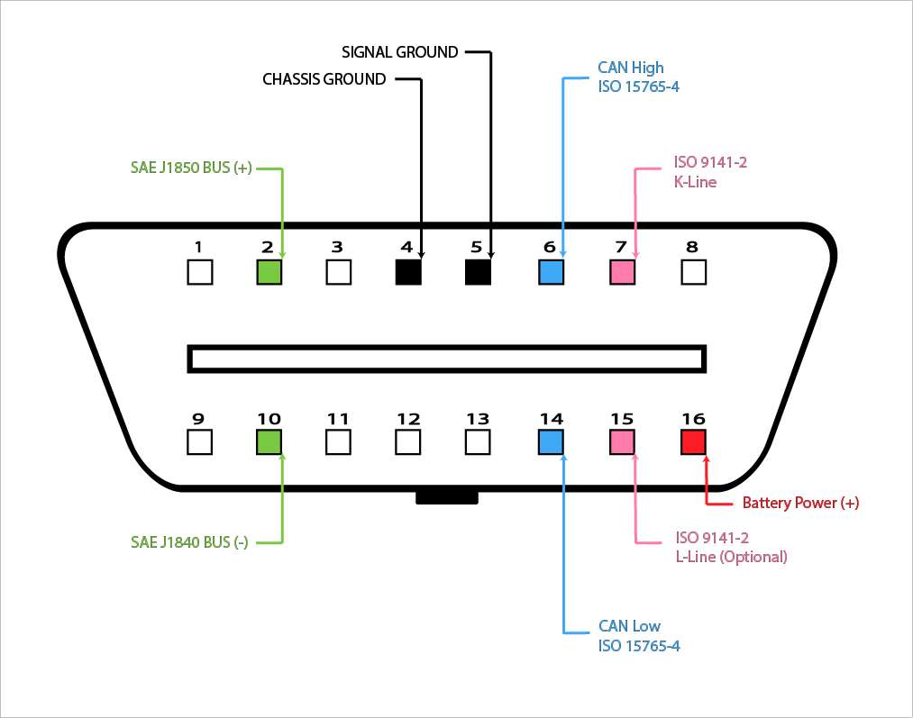
The Controller Area Network (CAN) bus is the nervous system of modern vehicles. Developed by Bosch in 1986, it's a multi-master serial bus where Electronic Control Units (ECUs) broadcast messages that any other ECU can receive.
CAN Message Structure
┌─────────────┬──────────┬─────────────┬──────────┬─────────┐
│ Arbitration │ Control  │    Data     │   CRC    │   ACK   │
│     ID      │  Field   │  (0-8 bytes)│  Field   │  Field  │
│  (11/29 bit)│          │             │          │         │
└─────────────┴──────────┴─────────────┴──────────┴─────────┘
A typical steering sensor message might look like:
ID: 0x14A (330 decimal)
Data: [0x00, 0x00, 0x0C, 0x80, 0x00, 0x00, 0x00, 0x00]
DBC Files: The Rosetta Stone
DBC (Database CAN) files define how to parse raw CAN bytes into meaningful values. From opendbc, here's a Honda steering sensor definition:
BO_ 330 STEERING_SENSORS: 8 EPS
 SG_ STEER_ANGLE : 7|16@0- (0.1,0) [-500|500] "deg" EON
 SG_ STEER_ANGLE_RATE : 23|8@0- (1,0) [-128|127] "deg/s" EON
 SG_ STEER_ANGLE_OFFSET : 39|8@0- (0.1,0) [-12.8|12.7] "deg" EON
This tells us:
- Message ID 330 contains steering data
STEER_ANGLEstarts at bit 7, is 16 bits, big-endian, signed, scaled by 0.1- The angle ranges from -500° to +500° (multiple steering wheel rotations)
Reading CAN Data in Python
openpilot's car interfaces parse CAN messages using generated code from DBC files:
# Simplified from openpilot's Honda interface
def update(self, can_packets):
    for cp in can_packets:
        # Parse steering angle from CAN message 0x14A
        self.steer_angle = cp.vl["STEERING_SENSORS"]["STEER_ANGLE"]

        # Parse vehicle speed from CAN message 0x158
        self.vehicle_speed = cp.vl["ENGINE_DATA"]["XMISSION_SPEED"] * CV.KPH_TO_MS

        # Parse brake pressure
        self.brake_pressed = cp.vl["POWERTRAIN_DATA"]["BRAKE_PRESSED"] == 1
Sending Control Commands
To steer the car, openpilot sends torque commands over CAN. Here's the conceptual flow:
# Simplified steering control message construction
def create_steering_control(steer_torque, steer_req, counter):
    values = {
        "STEER_TORQUE": steer_torque,        # -3840 to 3840
        "STEER_TORQUE_REQUEST": steer_req,   # 1 = requesting control
        "COUNTER": counter,                   # Rolling counter for safety
        "CHECKSUM": 0,                        # Calculated separately
    }
    return packer.make_can_msg("STEERING_CONTROL", 0, values)
The torque value doesn't specify where to turn the wheel—it specifies how hard to push. The control system closes the loop by continuously adjusting torque based on the actual vs. desired steering angle.
Safety: The Panda
The panda is comma.ai's CAN interface with built-in safety. When powered on, it starts in SAFETY_SILENT mode—unable to send any CAN messages. To enable control:
# Safety modes prevent unauthorized actuation
panda.set_safety_mode(Panda.SAFETY_HONDA_NIDEC)
Each safety mode enforces vehicle-specific limits:
- Maximum steering torque rate
- Steering only allowed when cruise engaged
- Brake/gas pedal override detection
- Watchdog timeouts
Localization
Before planning a path, the vehicle must know its precise position and orientation. GPS alone isn't sufficient—it's accurate to only ~2 meters and updates at just 1-10 Hz. Autonomous vehicles need centimeter-level accuracy at 100+ Hz.
Sensor Fusion with Extended Kalman Filter
The Extended Kalman Filter (EKF) fuses noisy measurements from multiple sensors into a coherent state estimate. It's the workhorse of robotics localization.
State vector (what we're estimating):
x = [position_x, position_y, position_z,
     velocity_x, velocity_y, velocity_z,
     orientation_roll, orientation_pitch, orientation_yaw,
     gyro_bias_x, gyro_bias_y, gyro_bias_z]
The EKF operates in two steps:
- Predict: Use IMU data (high rate, ~100Hz) to propagate state forward
- Update: Correct prediction when slower measurements arrive (GPS at 1Hz, camera odometry at 20Hz)
# Conceptual EKF implementation
class ExtendedKalmanFilter:
    def __init__(self):
        self.x = np.zeros(12)  # State vector
        self.P = np.eye(12)    # Covariance matrix

    def predict(self, imu_accel, imu_gyro, dt):
        # State transition using IMU
        # Integrate acceleration to get velocity
        # Integrate velocity to get position
        # Apply gyro rotation

        self.x = self.state_transition(self.x, imu_accel, imu_gyro, dt)

        # Update covariance (uncertainty grows)
        F = self.jacobian_of_transition(self.x, dt)
        self.P = F @ self.P @ F.T + self.Q  # Q = process noise

    def update(self, measurement, measurement_type):
        # Kalman gain determines how much to trust measurement
        H = self.measurement_jacobian(measurement_type)
        S = H @ self.P @ H.T + self.R  # R = measurement noise
        K = self.P @ H.T @ np.linalg.inv(S)

        # Correct state estimate
        y = measurement - self.measurement_model(self.x)  # Innovation
        self.x = self.x + K @ y
        self.P = (np.eye(12) - K @ H) @ self.P
openpilot's Localizer
openpilot's locationd service implements a PoseKalman filter fusing:
- Phone IMU (accelerometer + gyroscope)
- Camera-based visual odometry
- Vehicle speed from CAN bus
- GPS when available
# From openpilot locationd - observation integration
def handle_sensors(self, sensor_time, sensor_type, measurement):
    if sensor_type == ObservationKind.PHONE_ACCEL:
        # Accelerometer at ~100Hz
        self.kf.predict_and_observe(sensor_time,
                                     ObservationKind.PHONE_ACCEL,
                                     measurement)

    elif sensor_type == ObservationKind.CAMERA_ODO_ROTATION:
        # Visual odometry at 20Hz - validate first
        if self.validate_rotation(measurement):
            self.kf.predict_and_observe(sensor_time,
                                         ObservationKind.CAMERA_ODO_ROTATION,
                                         measurement)
The filter weights measurements by uncertainty. GPS is accurate to 2m but drifts slowly. IMU is precise short-term but accumulates drift. The Kalman filter combines them optimally.
Autoware's Localization Stack
Autoware uses a more sophisticated approach with multiple algorithms:
- NDT (Normal Distributions Transform): Matches LiDAR scans against HD map
- EKF: Fuses NDT pose with IMU and vehicle odometry
- Particle Filter: Alternative to EKF for non-Gaussian distributions
// Autoware EKF localization node (simplified)
void EKFLocalizer::callbackPose(const PoseWithCovariance::SharedPtr msg) {
    // Measurement from NDT matching
    Eigen::VectorXd y = poseMsgToEigen(msg);
    Eigen::MatrixXd R = covarianceMsgToEigen(msg->covariance);

    // EKF update step
    ekf_.update(y, R, measurement_model_);
}

void EKFLocalizer::callbackIMU(const Imu::SharedPtr msg) {
    // Predict step at IMU rate
    Eigen::VectorXd u = imuMsgToEigen(msg);
    ekf_.predict(u, dt_);
}
Perception
Perception transforms raw sensor data into a semantic understanding of the environment: other vehicles, pedestrians, lane lines, traffic signs, drivable space.
The Two Paradigms
Modular perception (Autoware, Apollo) separates tasks:
- Object detection → tracking → prediction
- Lane detection
- Traffic light classification
- Free space estimation
End-to-end perception (openpilot, Tesla FSD v12) uses a single neural network to output all driving-relevant information directly.
LiDAR Object Detection: PointPillars

For LiDAR-based systems, PointPillars is the standard architecture for real-time 3D object detection.
The problem: Point clouds are unordered and sparse. A 64-channel LiDAR produces ~100,000 points per scan, but they're not on a regular grid like image pixels.
PointPillars solution: Convert points into vertical columns ("pillars"), encode each pillar with a small PointNet, scatter to a 2D pseudo-image, then apply standard 2D convolutions.
# PointPillars architecture (simplified)
class PointPillars(nn.Module):
    def __init__(self):
        # Pillar Feature Net - encodes points within each pillar
        self.pfn = PillarFeatureNet(
            in_channels=9,  # x, y, z, intensity, x_c, y_c, z_c, x_p, y_p
            out_channels=64
        )

        # Backbone - 2D CNN on bird's eye view
        self.backbone = nn.Sequential(
            ConvBlock(64, 64, stride=1),
            ConvBlock(64, 128, stride=2),
            ConvBlock(128, 256, stride=2),
        )

        # Detection head - predicts boxes and classes
        self.head = DetectionHead(
            num_classes=3,  # car, pedestrian, cyclist
            num_anchors=2
        )

    def forward(self, pillars, coords):
        # Encode pillars
        features = self.pfn(pillars)  # (N, 64)

        # Scatter to pseudo-image
        pseudo_img = self.scatter(features, coords)  # (B, 64, H, W)

        # 2D backbone
        x = self.backbone(pseudo_img)

        # Detection
        return self.head(x)  # boxes, scores, classes
PointPillars runs at 62 Hz on a GPU—fast enough for real-time driving. VoxelNet, the predecessor, ran at just 4 Hz.
Camera Perception: Vision Transformers
openpilot's supercombo model processes camera images through a vision backbone followed by temporal aggregation.
Architecture evolution:
- 2021: EfficientNet backbone + GRU for temporal context
- 2024: FastViT (hybrid vision transformer) + improved temporal modeling
# Supercombo conceptual architecture
class Supercombo(nn.Module):
    def __init__(self):
        # Vision backbone - processes each frame
        self.backbone = FastViT_SA24()  # Hybrid CNN + Transformer

        # Feature Pyramid Network - multi-scale features
        self.fpn = BiFPN(channels=[64, 128, 256, 512])

        # Temporal aggregation - 5 seconds of context
        self.temporal = GRU(
            input_size=512,
            hidden_size=512,
            num_layers=1
        )

        # Output heads
        self.path_head = PathPredictionHead()      # Driving trajectory
        self.lane_head = LaneDetectionHead()       # Lane lines
        self.lead_head = LeadCarHead()             # Lead vehicle detection
        self.meta_head = MetaHead()                # Road type, etc.

    def forward(self, images, desire, traffic_convention):
        # images: (B, T, C, H, W) - batch of image sequences
        # desire: one-hot encoded driving intention
        # traffic_convention: left-hand vs right-hand drive

        B, T, C, H, W = images.shape

        # Extract features from each frame
        features = []
        for t in range(T):
            x = self.backbone(images[:, t])
            x = self.fpn(x)
            features.append(x)

        # Temporal aggregation
        features = torch.stack(features, dim=1)
        temporal_features, _ = self.temporal(features)

        # Predict outputs
        path = self.path_head(temporal_features[:, -1], desire)
        lanes = self.lane_head(temporal_features[:, -1])
        lead = self.lead_head(temporal_features[:, -1])

return path, lanes, leadInput: Two consecutive 256×512 RGB images at 20 Hz, plus:
- Desire vector (100 values = 5 seconds of commands)
- Traffic convention (left/right hand drive)
- Historical curvatures (100 previous predictions)
Output:
- Path plans for 33 timestamps over 10 seconds (192 meters)
- Lane line positions
- Lead vehicle distance and velocity
- Road edges
- Traffic light states
Tesla's Occupancy Networks
Tesla introduced a fundamentally different output representation in 2022: instead of detecting discrete objects with bounding boxes, predict occupancy of 3D space.
# Occupancy Network output (conceptual)
class OccupancyOutput:
    # 3D grid of occupancy probabilities
    occupancy_volume: Tensor  # (X, Y, Z) = (256, 256, 16)

    # Per-voxel velocity vectors
    occupancy_flow: Tensor    # (X, Y, Z, 3)

    # Semantic labels per voxel
    semantics: Tensor         # (X, Y, Z, num_classes)
Traditional object detection fails on novel objects (construction debris, fallen trees, animals). If the network wasn't trained on it, it won't detect it. Occupancy networks predict "something is here" regardless of object class.
Planning
Given localization and perception, the planner must generate a safe, comfortable trajectory to the goal.
Path Planning Hierarchy
Most systems use a hierarchical approach:
- Route Planning: Global path from A to B using road network (handled by maps)
- Behavioral Planning: High-level decisions (lane change, follow, stop)
- Motion Planning: Generate smooth, collision-free trajectories
- Trajectory Optimization: Refine for comfort and constraints
Model Predictive Control (MPC)
MPC is the dominant approach for trajectory optimization. It solves an optimization problem at each timestep:
# MPC formulation (conceptual)
def solve_mpc(current_state, reference_trajectory):
    """
    Minimize: Σ (x_t - x_ref)² + (u_t)²
    Subject to:
        x_{t+1} = f(x_t, u_t)   # Vehicle dynamics
        u_min ≤ u_t ≤ u_max    # Actuator limits
        x_t ∈ X_safe           # Collision avoidance
    """

    # State: [x, y, heading, velocity]
    # Control: [steering_angle, acceleration]

    N = 50  # Prediction horizon (e.g., 5 seconds at 10Hz)

    # Build optimization problem
    x = cp.Variable((4, N+1))
    u = cp.Variable((2, N))

    cost = 0
    constraints = [x[:, 0] == current_state]

    for t in range(N):
        # Tracking cost
        cost += cp.quad_form(x[:, t] - reference_trajectory[:, t], Q)

        # Control effort cost
        cost += cp.quad_form(u[:, t], R)

        # Dynamics constraint (bicycle model)
        constraints += [x[:, t+1] == vehicle_dynamics(x[:, t], u[:, t])]

        # Actuator constraints
        constraints += [u[0, t] >= -max_steer, u[0, t] <= max_steer]
        constraints += [u[1, t] >= -max_decel, u[1, t] <= max_accel]

    problem = cp.Problem(cp.Minimize(cost), constraints)
    problem.solve()

    return u[:, 0].value  # Return first control action
MPC re-plans at every timestep. If conditions change (car cuts in front), the next solve incorporates the new information.
openpilot's Approach: Learned Planning
openpilot 0.10 removed MPC entirely. Instead, the neural network directly outputs the desired trajectory, supervised during training by a "World Model" that simulates future outcomes.
# openpilot 0.10 planning (simplified)
def plan(self, model_output):
    # Neural network directly outputs trajectory
    # No optimization, no MPC—just network inference

    path = model_output.path  # 33 points over 10 seconds

    # Trajectory is (x, y) positions in vehicle frame
    # Already accounts for:
    # - Current speed
    # - Desired lane position
    # - Lead vehicle following
    # - Comfort constraints (learned from human drivers)

    return path
This is the "end-to-end" philosophy: train a network to directly map sensor inputs to control outputs, learning the entire pipeline implicitly.
Control
The control layer translates the planned trajectory into actual steering, throttle, and brake commands.
Lateral Control: Steering
PID Controller: The classic approach. Minimize cross-track error (distance from desired path).
class PIDLateralController:
    def __init__(self, kp=0.15, ki=0.0001, kd=1.0):
        self.kp = kp  # Proportional gain
        self.ki = ki  # Integral gain
        self.kd = kd  # Derivative gain

        self.integral = 0
        self.prev_error = 0

    def update(self, cross_track_error, dt):
        # P term: proportional to current error
        p_term = self.kp * cross_track_error

        # I term: accumulated error over time
        self.integral += cross_track_error * dt
        i_term = self.ki * self.integral

        # D term: rate of change of error
        derivative = (cross_track_error - self.prev_error) / dt
        d_term = self.kd * derivative

        self.prev_error = cross_track_error

        # Steering command
        steering = -(p_term + i_term + d_term)
        return np.clip(steering, -1.0, 1.0)
Why torque, not angle? At the actuator level, electric power steering (EPS) systems accept torque commands, not position commands. The PID loop runs at 100 Hz, continuously adjusting torque to track the desired steering angle.
openpilot's Control Loop
openpilot's controlsd runs at 100 Hz:
# From openpilot controlsd (simplified)
class Controls:
    def __init__(self):
        self.LaC = LatController()   # Lateral (steering)
        self.LoC = LongController()  # Longitudinal (speed)

    def control_loop(self):
        while True:
            # 1. Read current state
            self.update()  # From CAN bus and sensors

            # 2. Compute control commands
            steering_torque = self.LaC.update(
                self.desired_curvature,
                self.current_curvature,
                self.vehicle_speed
            )

            accel_command = self.LoC.update(
                self.desired_speed,
                self.current_speed,
                self.lead_car
            )

            # 3. Send commands to vehicle
            self.publish_controls(steering_torque, accel_command)

            # 4. Maintain 100Hz rate
            self.rate_keeper.keep_time()
Longitudinal Control: Speed
Adaptive Cruise Control (ACC) manages speed and following distance. The controller must balance:
- Tracking desired speed
- Maintaining safe following distance
- Smooth acceleration/deceleration
class LongitudinalController:
    def __init__(self):
        self.pid = PIDController(kp=1.0, ki=0.1, kd=0.0)

    def update(self, desired_speed, current_speed, lead_car):
        if lead_car.detected:
            # Following mode: maintain time gap
            desired_gap = self.time_gap * current_speed
            current_gap = lead_car.distance

            # Adjust desired speed based on gap error
            gap_error = current_gap - desired_gap
            speed_adjustment = self.gap_pid.update(gap_error)
            target_speed = min(desired_speed,
                              lead_car.speed + speed_adjustment)
        else:
            # Cruising mode: track desired speed
            target_speed = desired_speed

        # PID on speed error
        speed_error = target_speed - current_speed
        accel_command = self.pid.update(speed_error)

        return np.clip(accel_command, -3.0, 2.0)  # m/s²
Real-Time Constraints and Safety
Autonomous driving is a hard real-time system. Missing a control deadline can cause an accident. This demands specialized operating systems and architectures.
QNX: The Industry Standard
QNX Neutrino RTOS runs in over 275 million vehicles worldwide. Its microkernel architecture isolates every component:
┌─────────────────────────────────────────────────────────┐
│                     Applications                        │
├─────────────────────────────────────────────────────────┤
│  Perception  │  Planning  │  Control  │  Diagnostics   │
├─────────────────────────────────────────────────────────┤
│                    POSIX API                            │
├─────────────────────────────────────────────────────────┤
│  Network  │  Filesystem  │  Device Drivers  │  IPC     │
├─────────────────────────────────────────────────────────┤
│              QNX Neutrino Microkernel                   │
│        (Only kernel code runs in kernel space)          │
└─────────────────────────────────────────────────────────┘
If a driver or service crashes, it can be restarted without affecting the kernel or other services. In a monolithic kernel (Linux), a driver crash takes down the entire system.
QNX is certified to ISO 26262 ASIL D—the highest automotive safety level.
AUTOSAR: Standardized Architecture
AUTOSAR (AUTomotive Open System ARchitecture) provides a standardized software architecture for ECUs:
- Classic AUTOSAR: For hard real-time control (brake, steering)
- Adaptive AUTOSAR: For high-performance compute (ADAS, infotainment)
┌─────────────────────────────────────────────────────────┐
│              Application Software                       │
├─────────────────────────────────────────────────────────┤
│              Runtime Environment (RTE)                  │
├─────────────────────────────────────────────────────────┤
│  Services  │  ECU Abstraction  │  Complex Drivers      │
├─────────────────────────────────────────────────────────┤
│                 Microcontroller Abstraction             │
├─────────────────────────────────────────────────────────┤
│                     Microcontroller                     │
└─────────────────────────────────────────────────────────┘
Adaptive AUTOSAR runs on POSIX-compliant systems (QNX, Linux with PREEMPT_RT) and supports:
- Service-oriented communication
- Dynamic software updates (OTA)
- Machine learning inference
openpilot's Approach
openpilot runs on Android (Linux kernel) without hard real-time guarantees. It compensates with:
- Rate monitoring: Detect and log when control loops miss deadlines
- Graceful degradation: Disable autonomy if timing constraints aren't met
- Safety in hardware: The panda enforces watchdog timeouts—if commands stop, steering torque goes to zero
# From openpilot ratekeeper
class Ratekeeper:
    def __init__(self, rate, print_delay_threshold=None):
        self.rate = rate
        self.interval = 1.0 / rate
        self.print_delay_threshold = print_delay_threshold

    def monitor_time(self):
        current = time.monotonic()
        remaining = self.next_frame - current

        if remaining < 0:
            # Missed deadline
            if self.print_delay_threshold is not None:
                if -remaining > self.print_delay_threshold:
                    print(f"Control loop late by {-remaining*1000:.1f}ms")

        # Sleep until next frame
        if remaining > 0:
            time.sleep(remaining)

        self.next_frame += self.interval
Message Passing
Components in the autonomous stack must communicate efficiently. Two dominant approaches:
ROS 2 (Autoware)
ROS 2 uses DDS (Data Distribution Service) for publish-subscribe messaging with QoS guarantees:
// Autoware-style ROS 2 node
class PerceptionNode : public rclcpp::Node {
public:
    PerceptionNode() : Node("perception_node") {
        // Subscribe to point cloud from LiDAR driver
        lidar_sub_ = create_subscription<PointCloud2>(
            "/lidar/points",
            rclcpp::SensorDataQoS(),
            [this](PointCloud2::SharedPtr msg) {
                process_lidar(msg);
            }
        );

        // Publish detected objects
        objects_pub_ = create_publisher<DetectedObjects>(
            "/perception/objects",
            rclcpp::QoS(10)
        );
    }

private:
    void process_lidar(PointCloud2::SharedPtr cloud) {
        auto objects = detector_.detect(cloud);
        objects_pub_->publish(objects);
    }
};
ROS 2 provides real-time capabilities through:
- DDS-RTPS (Real-Time Publish-Subscribe)
- Configurable QoS (reliability, deadline, lifespan)
- Executor scheduling control
Custom IPC (openpilot)
openpilot uses a lightweight custom system: ZeroMQ for pub-sub, Cap'n Proto for serialization.
# openpilot messaging
import cereal.messaging as messaging

# Publisher
pm = messaging.PubMaster(['carState', 'carControl'])

while True:
    car_state = get_car_state()
    pm.send('carState', car_state)

# Subscriber
sm = messaging.SubMaster(['modelV2', 'carState', 'controlsState'])

while True:
    sm.update()
    if sm.updated['modelV2']:
        path = sm['modelV2'].position
openpilot's MSGQ (message queue) previously allocated 10MB per service, growing to 711MB total. A 2024 optimization reduced this to 90MB with per-service configurable buffers.
End-to-End Learning
Traditional Modular Stack
Camera → Object Detection → Tracking → Prediction → Planning → Control
         ↓
LiDAR  → Point Cloud Processing →
         ↓
Radar  → Sensor Fusion →
Each module is trained/tuned independently. Errors compound through the pipeline.
End-to-End Learning
Tesla's FSD v12 and openpilot 0.10 collapse this into:
Cameras → Neural Network → ControlWhat this means technically:
- Training: Network supervised on human driving demonstrations
- Loss function: Imitation learning—minimize deviation from human actions
- World model: Learns physics, object behavior implicitly
openpilot 0.10 training uses a "World Model" that predicts future states:
# Conceptual training loop
def train_step(images, human_trajectory):
    # Forward pass through driving model
    predicted_trajectory = model(images)

    # World model simulates consequences of predicted trajectory
    simulated_future = world_model.simulate(predicted_trajectory)

    # Loss: how close is simulated future to actual future?
    loss = trajectory_loss(predicted_trajectory, human_trajectory)
    loss += collision_loss(simulated_future)
    loss += comfort_loss(predicted_trajectory)

    loss.backward()
    optimizer.step()
Trade-offs
| Aspect | Modular | End-to-End |
|---|---|---|
| Interpretability | High—can inspect each module | Low—black box |
| Data requirements | Moderate | Massive (Tesla: 1.5 PB) |
| Handling edge cases | Explicit rules | Must be in training data |
| Development iteration | Slow (retest each module) | Fast (retrain model) |
| Compute requirements | Distributed across ECUs | Centralized GPU |
Full Data Flow
Here's the complete data flow for openpilot processing a single frame:
1. CAMERA CAPTURE (visionipc)
   ├── Road camera: 1164x874 @ 20Hz
   └── Driver camera: 1152x864 @ 20Hz

2. PERCEPTION (modeld)
   ├── Input: 2 consecutive frames + state
   ├── Model: FastViT + GRU (supercombo)
   ├── Output: path, lanes, leads, road edges
   └── Latency: ~25ms on comma 3X

3. LOCALIZATION (locationd)
   ├── Input: IMU @ 100Hz, camera odo @ 20Hz, GPS @ 1Hz
   ├── Algorithm: Extended Kalman Filter
   ├── Output: position, velocity, orientation
   └── Latency: <1ms per update

4. PLANNING (plannerd)
   ├── Input: model output, localization, map
   ├── Algorithm: Neural network (no MPC in 0.10)
   └── Output: desired trajectory

5. CONTROL (controlsd) @ 100Hz
   ├── Input: desired trajectory, vehicle state
   ├── Lateral: torque-based PID on curvature
   ├── Longitudinal: PID on speed/distance
   └── Output: steering torque, acceleration

6. ACTUATION (pandad)
   ├── Input: control commands
   ├── Safety checks: rate limits, watchdog
   └── Output: CAN messages to vehicle
Total latency from camera to wheel: ~100ms
This is fast enough because the system predicts 10 seconds ahead. By the time the prediction executes, it's still valid.
Where to Learn More
Open Source Codebases
- openpilot: End-to-end stack, Python/C++
- opendbc: CAN database for 500+ vehicles
- Autoware: Modular ROS 2 stack
- Apollo: Baidu's modular stack
- CARLA: Open source simulator
Key Papers
- PointPillars - Real-time LiDAR detection
- Attention Is All You Need - Transformers
- End to End Learning for Self-Driving Cars - NVIDIA's seminal work
comma.ai Resources
Where This Is Going
End-to-end learning is replacing hand-crafted modules. Vision is replacing LiDAR. Foundation models trained on internet-scale data are entering the loop.
The fundamentals remain: sense the world, understand it, plan a path, execute it safely. The implementations change; the problem doesn't.